In order to study diseases such as leukaemia on cell populations level, we first need to characterise a healthy bone marrow cell population. So in this blog we set out to do just that.
The data from Galen et al.(Cell, 2019) is available in the GEO database under the accession number GSE116256. We will be using the data from only one healthy person BM4 and its annotation file since this is by far the biggest nonenriched sample from a healthy individual in this dataset.
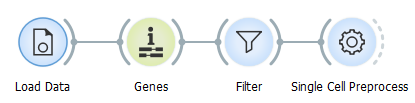
After we load the data (alternatively, you can load the Healthy human bone marrow dataset using the Single Cell Datasets widget) and match the genes in the dataset to those in databases, we filter out all the genes that appear in less than 10 cells. Besides the usual normalisation, we select the 5000 most variable genes.
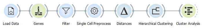
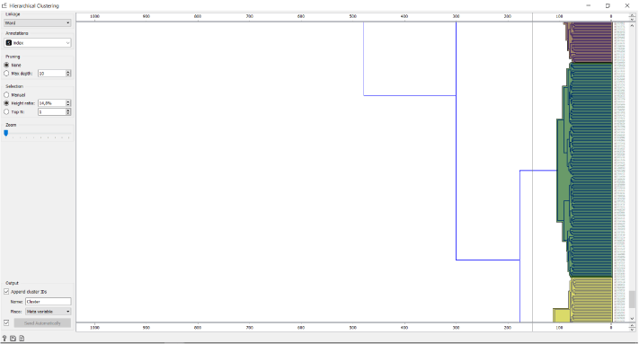
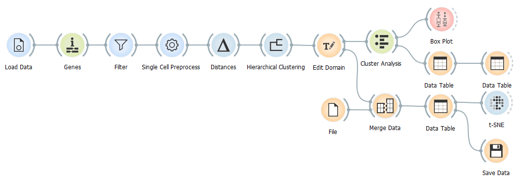
Since the relationships between the cell clusters is important for this analysis, we use the Hierarhical Clustering and not the Louvian Clustering widget to cluster the data. Firstly, we calculate the distances between the cells and then visually determine the number of clusters by dragging the vertical line over the graph.
We can tackle the identification of the clusters using two different approaches. The first is identifying the most significant genes in each cluster as described in one of our previous blogs and assuming cell types according to marker genes’ functions, the other is using the annotation file provided by Galen et al..
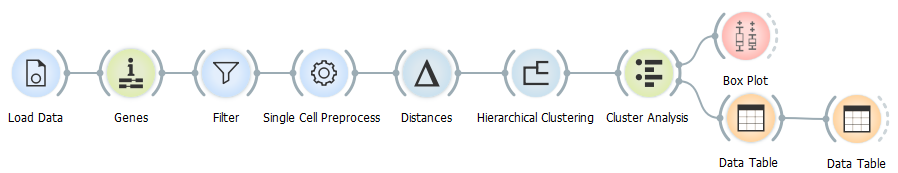
But before we take a closer look at either of the alternatives, let us take a look at the distribution of the clusters using the Box Plot widget.
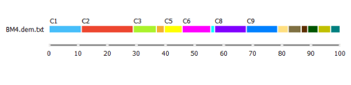
C2 is the biggest cluster. This information might come in handy when we try to identify them.
What we have also already done in this workflow, is identified markers for each cluster with the help of the Data Tables (explained in detail in this blog). With these markers we can classify clusters. For example, CD3D is the most significant gene in cluster 4. It encodes T-cell surface glycoprotein CD3. Similarly MS4A1 in the cluster 3 encodes B-lymphocyte antigen CD20.
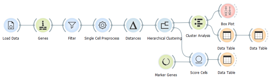
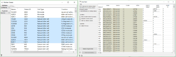
In case we run into problems identifying genes with this approach, we can always use the Score Cells widget to classify cells using known gene markers. Select the genes for the desired cell type, which are conveniently available in the Marker Genes widget, and then order them by score in a new Data Table widget. As we can see in this case, most of the highly scored cells for natural killer cell markers show up in C1.
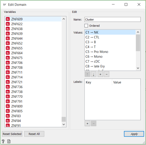
Now that we have matched clusters with the cell types, we can use the Edit Domain widget to change annotations of the clusters.
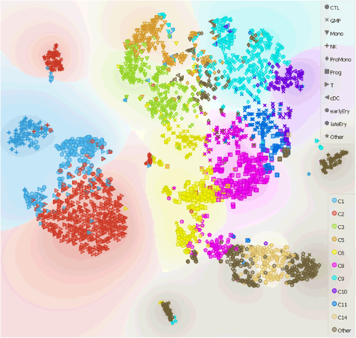
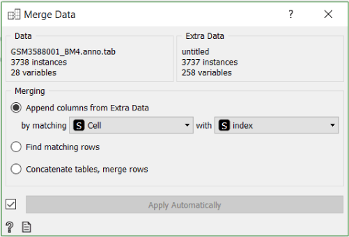
Additionally, we can merge the annotation file provided by Galen et al. with our data and display both cell classifications on t-SNE projection simultaneously.
To make the annotation file readable to Orange, we need to rename it from GSM3588001_BM4.anno.txt.gz to GSM3588001_BM4.anno.tab.gz. After that we can load it and merge it with our data using the Merge Data widget.
Have you noticed that we did not use the Cluster Analysis widget as our output for the data we are about to display using t-SNE? This is because it reduces the data and therefore negatively influences our t-SNE visualisation, therefore we used the Edit Domain widget as out output for the data.
Lets check how our clustering and cell identification compares to that of Galen et al..
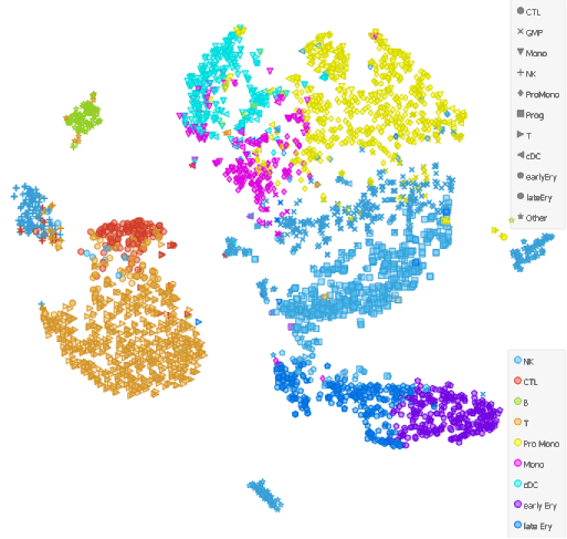
Apart from some mismatches along the putative cell differentiation trajectories (for example with the Progenitor Monocytes and the Monocytes along the continuum of cells from HSCs to monocytes), cell types overlap.
So, we have achieved what we undertook; characterised the human bone marrow cell population and displayed cell differentiation trajectories on t-SNE projection.
References
Van Galen P, Hovestadt V, Wadsworth MH, et al. (2016). Single-Cell RNA-Seq Reveals AML Hierarchies Relevant to Disease Progression and Immunity. Cell, 176(6), 1265–1281.